Data normalization and merging strategies differentially impact the measured batch effect
Benjamin R Babcock
NormalizationMethods.RmdLog-Normalize + Scaling (Figure 5A)
Prior to merging (individual samples)
Data filtering & normalization
library(BatchNorm)
# Import unfiltered Seurat object (included with 'BatchNorm' package)
data(PBMCs)

# Filter sample by mitochondrial percentage (+5 SD)
PBMCs <- MitoFilter(PBMCs)
# Run "standard" Seurat workflow on a list of samples, independently:
# Including data normalization, variable gene selection and gene scaling (performed on each sample individually, prior to merging samples for joint analysis)
PBMCs.list <- SplitObject(PBMCs, split.by = "orig.ident")
features.list <- list()
# Normalize data & select highly variable transcripts
for (i in 1:length(PBMCs.list)) {
    PBMCs.list[[i]] <- PBMCs.list[[i]] %>%
                       NormalizeData(normalization.method = "LogNormalize",
                                     assay = "RNA", scale.factor = 10000) %>%
                       NormalizeData(normalization.method = "CLR",
                                     assay = "ADT") %>%
                       FindVariableFeatures(selection.method = "vst",
                                            nfeatures = 2000)
    features.list[[i]] <- PBMCs.list[[i]]@assays$RNA@var.features
}
# Merge into a cohesive list of variable transcripts, keeping only those which are shared between all individual lists
var.features <- Reduce(intersect, list(features.list[[1]],
                                   features.list[[2]],
                                   features.list[[3]]))
# Merge all three samples into a single object for joint analysis of cells
PBMCs <- merge(PBMCs.list[[1]], y = c(PBMCs.list[[2]], PBMCs.list[[3]]),
               project = "PBMCs")
# Update variable genes in object
PBMCs@assays$RNA@var.features <- var.features
# Scale data and generate PBMCs
PBMCs <- PBMCs %>%
         ScaleData() %>%
         RunPCA(npcs = 30)
Selecting the appropriate number of Principal Components for UMAP reduction
## Identify correct numbers of PCs
## (Takes up to 5 minutes. Not run while rendering vignette for time)

# PBMCs.pca.test <- TestPCA(PBMCs)
# PBMCs.pca.test[, 1:20]

## 9 PCs with z > 1
## Proceed with 9 PCs for dimensional reduction & clustering
## Visualize PCs plotted by standard deviation:
ElbowPlot(PBMCs)
Generating a UMAP and clusters
PBMCs <- PBMCs %>%
         RunUMAP(reduction = "pca", dims = 1:9) %>%
         FindNeighbors(reduction = "pca", dims = 1:9) %>%
         FindClusters(resolution = .8)
## Modularity Optimizer version 1.3.0 by Ludo Waltman and Nees Jan van Eck
##
## Number of nodes: 16946
## Number of edges: 551155
##
## Running Louvain algorithm...
## Maximum modularity in 10 random starts: 0.8846
## Number of communities: 14
## Elapsed time: 2 seconds
UMAPPlot(PBMCs, cols = colors.use, group.by = "orig.ident") + ggtitle("Log-Normalize + Scale (Prior to merging) \nSample ID")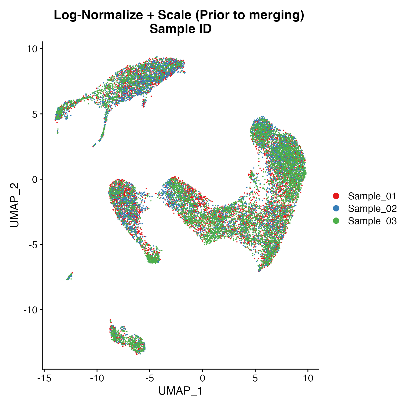
Measuring sample-UMAP integration (generating an iLISI score)
GetiLISI(object = PBMCs, nSamples = 3)## [1] 0.210613Cell Typing of joint PBMCs object for CMS
Convert cluster classifications to cell type classifications
# For complete cell classification workflow see our vignette "Biaxial Gating of a Single Sample"
# More details can be found in figure S3 of our manuscript "Data Matrix Normalization and Merging Strategies Minimize Batch-specific Systemic Variation in scRNA-Seq Data."
UMAPPlot(PBMCs, cols = colors.use, pt.size = 2,
         group.by = "seurat_clusters", label = T) + ggtitle("Log-Normalize + Scale (Prior to merging) \nClusters")
# B_Cells = 8
# T_CD4 = 0, 1, 13
# No TReg: Within cluster 1
# T_CD8 = 2, 7
# NK_T = 5
# NK = 3
# NK_CD56Hi = 10
# Monocyte_Classical = 4, 6
# Monocyte_NonClassical = 9
# Dendritic_Cells = 11, 12
# HSPCs = no cluster
# Cycling_Cells = no cluster
Idents(PBMCs) <- PBMCs[["seurat_clusters"]]
Idents(PBMCs) <- plyr::mapvalues(Idents(PBMCs), from = c(8, 0, 1, 13,
                                                         2, 7, 5, 3, 10,
                                                         4, 6,
                                                         9, 11, 12),
                to = c('B_Cells', 'T_CD4', 'T_CD4', 'T_CD4',
                       'T_CD8', 'T_CD8', 'NK_T', "NK", "NK_CD56Hi",
                       'Monocyte_Classical', 'Monocyte_Classical',
                       'Monocyte_NonClassical', 'Dendritic_Cells', 'Dendritic_Cells'))
Idents(PBMCs) <- factor(Idents(PBMCs),
                                 levels = c("B_Cells", "T_CD4", "TReg",
                                            "T_CD8", "NK_T", "NK", "NK_CD56Hi",
                                            "Monocyte_Classical", "Monocyte_NonClassical",
                                            "Dendritic_Cells", "HSPCs", "Cycling_Cells"))
PBMCs[["Cell_Type"]] <- Idents(PBMCs)
UMAPPlot(PBMCs, cols = colors.use, label = F) + ggtitle("Log-Normalize + Scale (Prior to merging) \nCell type classifications")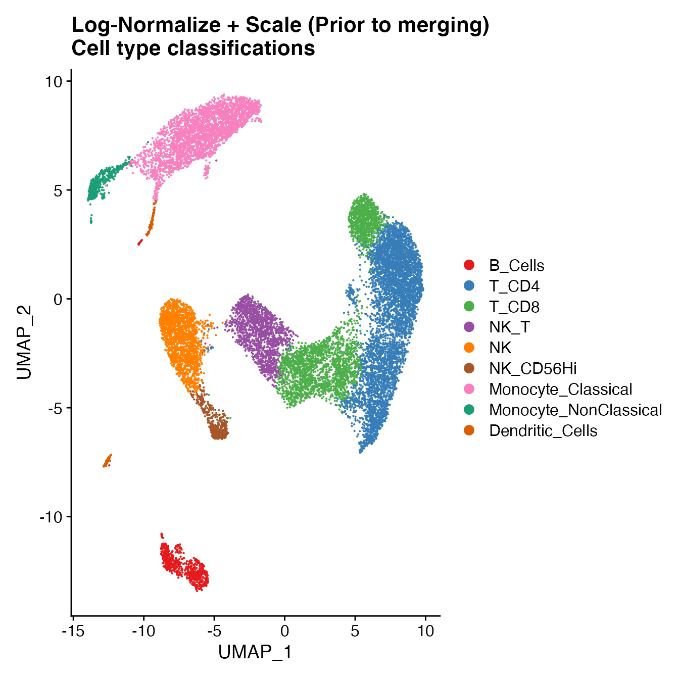
Compare single-sample workflow cell type classifications to joint classifications (generating a CMS)
# PBMC Sample 1
data(PBMC1_Single_ID)
S1cms <- GetCMS(object = PBMCs,
                sample.ID = "Sample_01",
                reference.ID = PBMC1_Single_ID)
# PBMC Sample 2
data(PBMC2_Single_ID)
S2cms <- GetCMS(object = PBMCs,
                sample.ID = "Sample_02",
                reference.ID = PBMC2_Single_ID)
# PBMC Sample 3
data(PBMC3_Single_ID)
S3cms <- GetCMS(object = PBMCs,
                sample.ID = "Sample_03",
                reference.ID = PBMC3_Single_ID)

# Average CMS
mean(c(S1cms, S2cms, S3cms))
## [1] 0.1598935Log-Normalize + Scaling (Figure 5A)
After merging (joined samples)
# This is an identical workflow to that presented in the vignette titled "Sample Donor Effects (Figure 2A)."
# For brevity, I have not duplicated this workflow again here.
# To see details on that analysis (the results of which are also summarised in figure 5A, right panel) please view that vignette and our manuscript.
SCTransform normalization (Figure 5B)
Prior to merging (individual samples)
Data filtering & normalization
library(BatchNorm)
# Import unfiltered Seurat object (included with 'BatchNorm' package)
data(PBMCs)

# Filter sample by mitochondrial percentage (+5 SD)
PBMCs <- MitoFilter(PBMCs)
# Run "standard" Seurat workflow on a list of samples, independently:
# Including data normalization, variable gene selection and gene scaling (performed on each sample individually, prior to merging samples for joint analysis)
PBMCs.list <- SplitObject(PBMCs, split.by = "orig.ident")
features.list <- list()
# Apply SCTransform to normalize data & select highly variable transcripts
for (i in 1:length(PBMCs.list)) {
    PBMCs.list[[i]] <- PBMCs.list[[i]] %>%
                       MitoFilter() %>%
                       NormalizeData(verbose = FALSE, assay = "ADT",
                                     normalization.method = "CLR") %>%
                       SCTransform(verbose = FALSE) %>%
                       RunPCA(npcs = 30)
    features.list[[i]] <- PBMCs.list[[i]]@assays$SCT@var.features
}
# Merge into a cohesive list of variable transcripts, keeping only those which are shared between all individual lists
var.features <- Reduce(intersect, list(features.list[[1]],
                                   features.list[[2]],
                                   features.list[[3]]))
# Merge all three samples into a single object for joint analysis of cells
PBMCs <- merge(PBMCs.list[[1]], y = c(PBMCs.list[[2]], PBMCs.list[[3]]),
               project = "PBMCs")
# Update variable genes in object
PBMCs@assays$SCT@var.features <- var.features
# Scale data and generate PBMCs
PBMCs <- PBMCs %>%
         RunPCA(npcs = 30, assay = "SCT")
Selecting the appropriate number of Principal Components for UMAP reduction
## Identify correct numbers of PCs
## (Takes up to 5 minutes. Not run while rendering vignette for time)

# PBMCs.pca.test <- TestPCA(genes.use = PBMCs@assays$SCT@var.features,
#                           mtx.use = PBMCs@assays$SCT@scale.data)
# PBMCs.pca.test[, 1:20]

## 9 PCs with z > 1
## Proceed with 9 PCs for dimensional reduction & clustering
## Visualize PCs plotted by standard deviation:
ElbowPlot(PBMCs)
Generating a UMAP and clusters
PBMCs <- PBMCs %>%
         RunUMAP(reduction = "pca", dims = 1:9) %>%
         FindNeighbors(reduction = "pca", dims = 1:9) %>%
         FindClusters(resolution = .8)
## Modularity Optimizer version 1.3.0 by Ludo Waltman and Nees Jan van Eck
##
## Number of nodes: 16887
## Number of edges: 541494
##
## Running Louvain algorithm...
## Maximum modularity in 10 random starts: 0.8892
## Number of communities: 18
## Elapsed time: 2 seconds
UMAPPlot(PBMCs, cols = colors.use, group.by = "orig.ident") + ggtitle("SCTransform (Prior to merging) \nSample ID")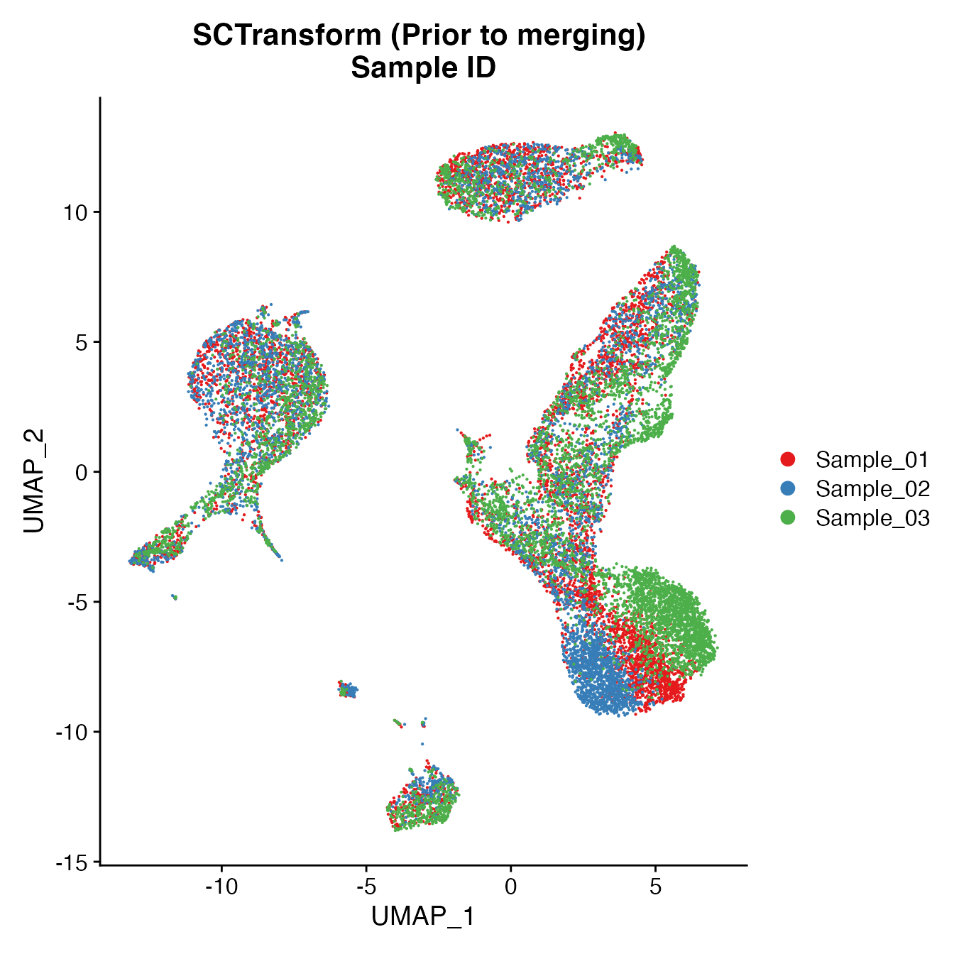
Measuring sample-UMAP integration (generating an iLISI score)
GetiLISI(object = PBMCs, nSamples = 3)## [1] 0.4156777Cell Typing of joint PBMCs object for CMS
Convert cluster classifications to cell type classifications
# For complete cell classification workflow see our vignette "Biaxial Gating of a Single Sample"
# More details can be found in figure S3 of our manuscript "Data Matrix Normalization and Merging Strategies Minimize Batch-specific Systemic Variation in scRNA-Seq Data."
UMAPPlot(PBMCs, cols = colors.use, pt.size = 2,
         group.by = "seurat_clusters", label = T) + ggtitle("SCTransform (Prior to merging) \nClusters")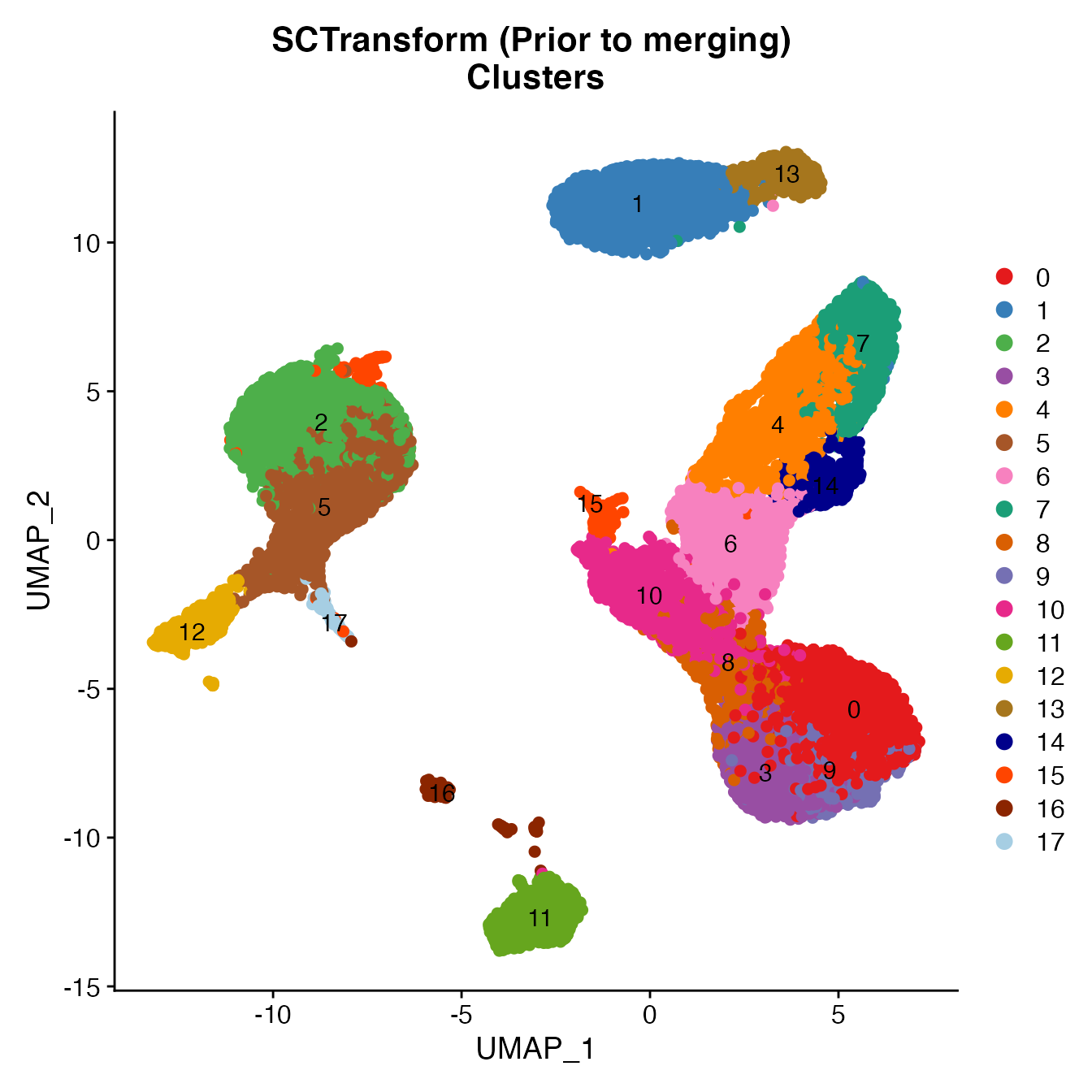
# B_Cells = 11
# T_CD4 = 0, 6, 8, 10, 15
# No TReg: Within cluster 10
# T_CD8 = 3, 4, 9, 14
# NK_T = 7
# NK = 1
# NK_CD56Hi = 13
# Monocyte_Classical = 2, 5
# Monocyte_NonClassical = 12
# Dendritic_Cells = 16, 17
# HSPCs = no cluster
# Cycling_Cells = no cluster
Idents(PBMCs) <- PBMCs[["seurat_clusters"]]
Idents(PBMCs) <- plyr::mapvalues(Idents(PBMCs), from = c(11, 0, 6, 8, 10, 15,
                                                         3, 4, 9, 14, 7,
                                                         1, 13,
                                                         2, 5,
                                                         12, 16, 17),
                to = c('B_Cells', 'T_CD4', 'T_CD4', 'T_CD4', 'T_CD4', 'T_CD4',
                       'T_CD8', 'T_CD8', 'T_CD8', 'T_CD8', 'NK_T',
                       "NK", "NK_CD56Hi",
                       'Monocyte_Classical', 'Monocyte_Classical',
                       'Monocyte_NonClassical', 'Dendritic_Cells', 'Dendritic_Cells'))
Idents(PBMCs) <- factor(Idents(PBMCs),
                                 levels = c("B_Cells", "T_CD4", "TReg",
                                            "T_CD8", "NK_T", "NK", "NK_CD56Hi",
                                            "Monocyte_Classical", "Monocyte_NonClassical",
                                            "Dendritic_Cells", "HSPCs", "Cycling_Cells"))
PBMCs[["Cell_Type"]] <- Idents(PBMCs)
UMAPPlot(PBMCs, cols = colors.use, label = F) + ggtitle("SCTransform (Prior to merging) \nCell type classifications")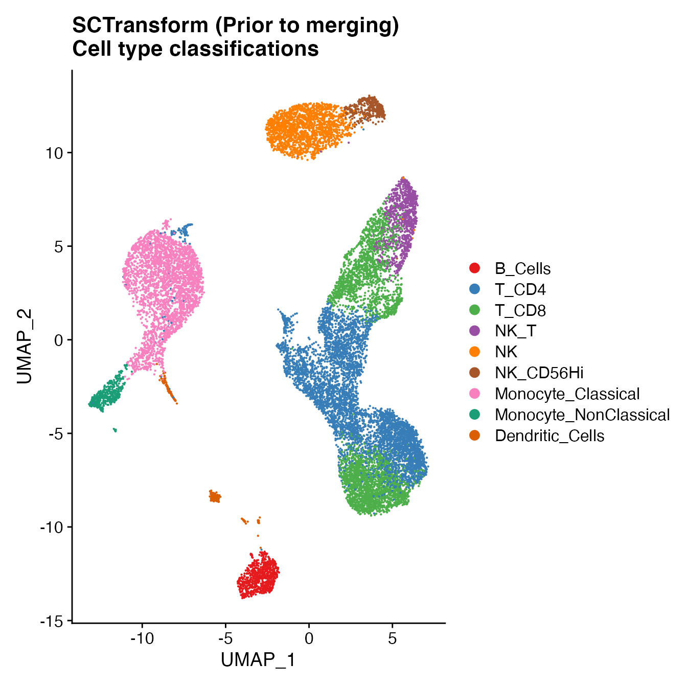
Compare single-sample workflow cell type classifications to joint classifications (generating a CMS)
# PBMC Sample 1
data(PBMC1_Single_ID)
S1cms <- GetCMS(object = PBMCs,
                sample.ID = "Sample_01",
                reference.ID = PBMC1_Single_ID)
# PBMC Sample 2
data(PBMC2_Single_ID)
S2cms <- GetCMS(object = PBMCs,
                sample.ID = "Sample_02",
                reference.ID = PBMC2_Single_ID)
# PBMC Sample 3
data(PBMC3_Single_ID)
S3cms <- GetCMS(object = PBMCs,
                sample.ID = "Sample_03",
                reference.ID = PBMC3_Single_ID)

# Average CMS
mean(c(S1cms, S2cms, S3cms))
## [1] 0.2020373SCTransform normalization (Figure 5B)
After merging (joined samples)
Data filtering & normalization
library(BatchNorm)
# Import unfiltered Seurat object (included with 'BatchNorm' package)
data(PBMCs)

# Run "standard" Seurat workflow: "https://satijalab.org/seurat/articles/pbmc3k_tutorial.html"
# Including a filter of sample by mitochondrial percentage (+5 SD)
PBMCs <- PBMCs %>%
         MitoFilter() %>%
         NormalizeData(verbose = FALSE, assay = "ADT", normalization.method = "CLR") %>%
         SCTransform(verbose = FALSE) %>%
         RunPCA(npcs = 30)
Selecting the appropriate number of Principal Components for UMAP reduction
## Identify correct numbers of PCs
## (Takes up to 5 minutes. Not run while rendering vignette for time)

# PBMCs.pca.test <- TestPCA(genes.use = PBMCs@assays$SCT@var.features,
#                           mtx.use = PBMCs@assays$SCT@scale.data)
# PBMCs.pca.test[, 1:20]

## 14 PCs with z > 1
## Proceed with 14 PCs for dimensional reduction & clustering
## Visualize PCs plotted by standard deviation:
ElbowPlot(PBMCs)
Generating a UMAP and clusters
PBMCs <- PBMCs %>%
         RunUMAP(reduction = "pca", dims = 1:14) %>%
         FindNeighbors(reduction = "pca", dims = 1:14) %>%
         FindClusters(resolution = .8)
## Modularity Optimizer version 1.3.0 by Ludo Waltman and Nees Jan van Eck
##
## Number of nodes: 16946
## Number of edges: 574465
##
## Running Louvain algorithm...
## Maximum modularity in 10 random starts: 0.8858
## Number of communities: 18
## Elapsed time: 2 seconds
UMAPPlot(PBMCs, cols = colors.use, group.by = "orig.ident") + ggtitle("SCTransform (After merging) \nSample ID")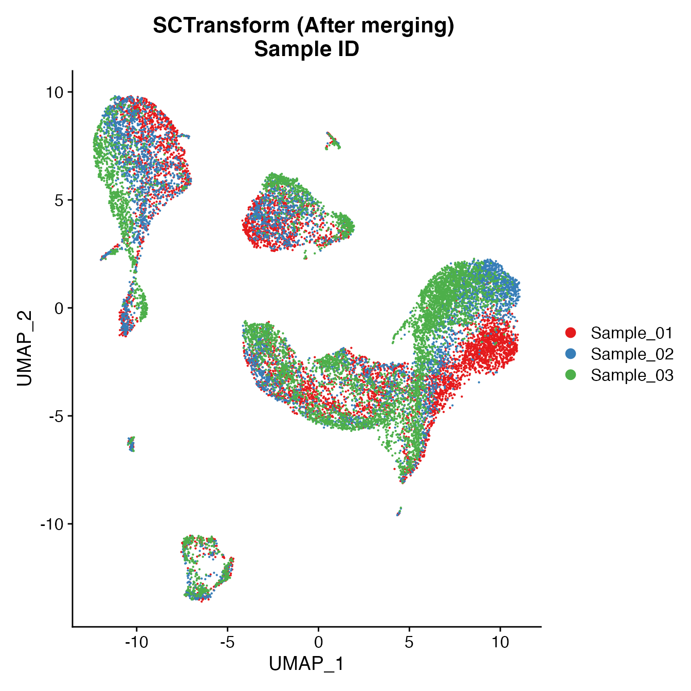
Measuring sample-UMAP integration (generating an iLISI score)
GetiLISI(object = PBMCs, nSamples = 3)## [1] 0.5585073Cell Typing of joint PBMCs object for CMS
Convert cluster classifications to cell type classifications
# For complete cell classification workflow see our vignette "Biaxial Gating of a Single Sample"
# More details can be found in figure S3 of our manuscript "Data Matrix Normalization and Merging Strategies Minimize Batch-specific Systemic Variation in scRNA-Seq Data."
UMAPPlot(PBMCs, cols = colors.use, pt.size = 2,
         group.by = "seurat_clusters", label = T) + ggtitle("SCTransform (After merging) \nClusters")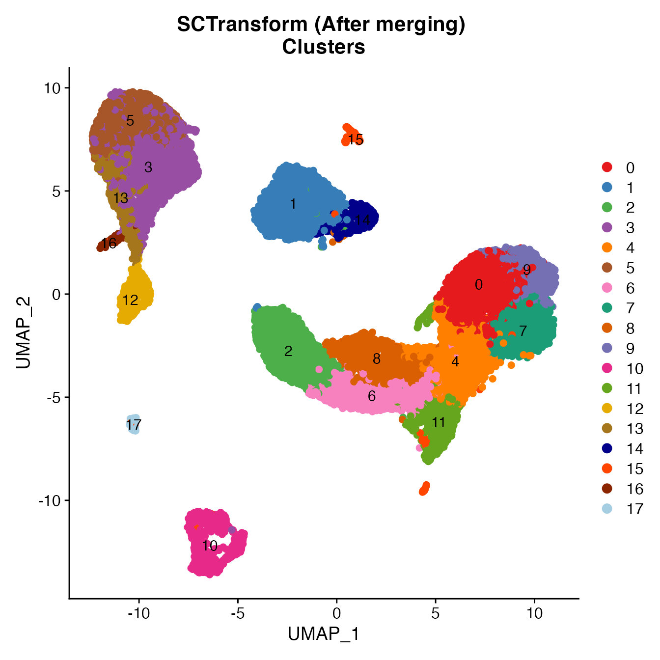
# B_Cells = 10
# T_CD4 = 0, 4
# TReg = 11
# T_CD8 = 6, 7, 8, 9
# NK_T = 2
# NK = 1
# NKCD56Hi = 14
# Monocyte_Classical = 3, 5, 13
# Monocyte_NonClassical = 12
# Dendritic_Cells = 16, 17
# HSPCs = 15
# No Cycling_Cells. Within NK cluster
Idents(PBMCs) <- PBMCs[["seurat_clusters"]]
Idents(PBMCs) <- plyr::mapvalues(Idents(PBMCs), from = c(10, 0, 4, 11, 6,
                                                         7, 8, 9, 2, 1, 14,
                                                         3, 5, 13,
                                                         12, 16, 17,
                                                         15),
                to = c('B_Cells', 'T_CD4', 'T_CD4', 'TReg', 'T_CD8',
                       'T_CD8', 'T_CD8', 'T_CD8', 'NK_T', "NK", 'NK_CD56Hi',
                       'Monocyte_Classical', 'Monocyte_Classical', 'Monocyte_Classical',
                       'Monocyte_NonClassical', 'Dendritic_Cells', 'Dendritic_Cells',
                       'HSPCs'))
Idents(PBMCs) <- factor(Idents(PBMCs),
                                 levels = c("B_Cells", "T_CD4", "TReg",
                                            "T_CD8", "NK_T", "NK", "NK_CD56Hi",
                                            "Monocyte_Classical", "Monocyte_NonClassical",
                                            "Dendritic_Cells", "HSPCs", "Cycling_Cells"))
PBMCs[["Cell_Type"]] <- Idents(PBMCs)
UMAPPlot(PBMCs, cols = colors.use, label = F) + ggtitle("SCTransform (After merging) \nCell type classifications")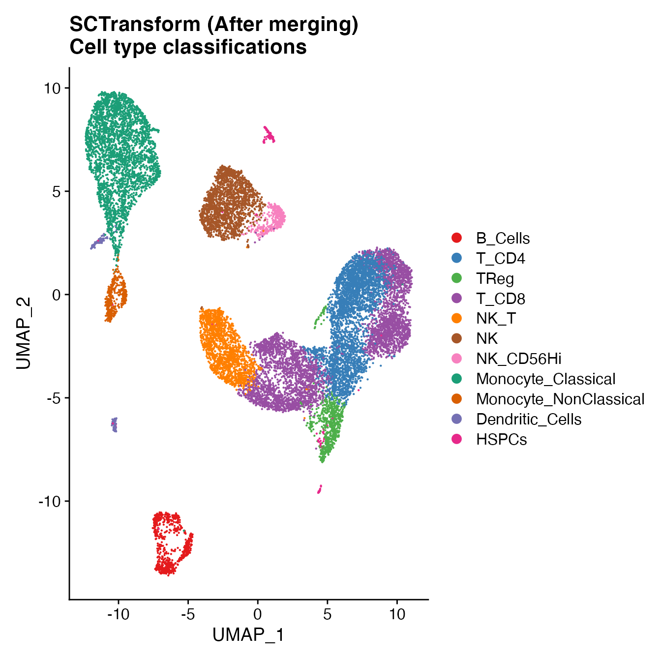
Compare single-sample workflow cell type classifications to joint classifications (generating a CMS)
# PBMC Sample 1
data(PBMC1_Single_ID)
S1cms <- GetCMS(object = PBMCs,
                sample.ID = "Sample_01",
                reference.ID = PBMC1_Single_ID)
# PBMC Sample 2
data(PBMC2_Single_ID)
S2cms <- GetCMS(object = PBMCs,
                sample.ID = "Sample_02",
                reference.ID = PBMC2_Single_ID)
# PBMC Sample 3
data(PBMC3_Single_ID)
S3cms <- GetCMS(object = PBMCs,
                sample.ID = "Sample_03",
                reference.ID = PBMC3_Single_ID)

# Average CMS
mean(c(S1cms, S2cms, S3cms))
## [1] 0.2040421